The first step in the Analysis Mode is to click ”Filename” to specify the name of the file that will contain the commands needed for the analysis. This file may be an existing one or it may be a new one to be created. It will be written as a text file. Conventionally, we have used ”con” as the file extension for this command file, but it is not required.
If the specified ”con” file is new, the ”Analysis” button will not be enabled until the ”Setup” has completed. Similarly, the ”Output” and ”Graph” buttons will not be enabled until the analysis calculations are completed. If the specified ”con” file already exists, the ”Analysis” button will already be enabled. However, the ”Setup” function can still be used to either view or change the settings. Also, if the analysis calculations were previously completed for the specified ”con” file, the ”Output” and ”Graph” buttons buttons will already be enabled.
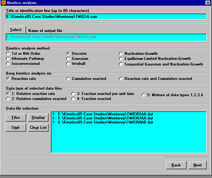
Clicking the ”Setup” button in the above window, will display the following window. The first step is to enter the Title or identification line to be used in the output files. By default this line is simply the file path and file name of the input command file, but it may be changed. The second step is to use the ”Select” button to enter the name of the output text file. Conventionally, we have used ”out” as the file extension for this file, but it is not required.
There are a nine principal kinetics analysis models that can be used. These are discussed in the Features window. Selection of the most appropriate model can be based on simply trying different methods to find the one with the best fit. Regardless of which model is selected, various other approximate methods are also used and displayed before the selected method is actually done. The approximate methods can give additional guidance in choosing the most appropriate analysis method, as will be illustrated later. More generally, however, past experience in analyzing a similar type of data will be the best guide. Petroleum source rocks are usually analyzed most successfully with the ”Discrete” model, i.e., using a single frequency factor and a discrete distribution of activation energies. This is the method we have selected for analysis of the Monterey data.
The kinetics analysis can be based on reaction rate, cumulative reacted, or both. The choice is usually, but not necessarily, the same as the data type. For example, if the data type is reaction rate, one might sometimes be interested in getting the best fit for the cumulative reacted values and, therefore, would base the kinetics analysis on cumulative reacted or possibly on both reaction rate and cumulative reacted.
There are four main types of data. Types 1 and 2 are ”relative” in the sense of involving an arbitrary scale factor. Types 3 and 4 can be considered ”absolute”, with the fraction reacted ranging from 0 as the start of the reaction to 1 at the completion of the reaction. In the analysis of ”relative” data, a scale factor is automatically determined to place the data on an absolute scale as best as possible. Kinetics05 does allow a mixture of the four data type to be simultaneously analyzed.
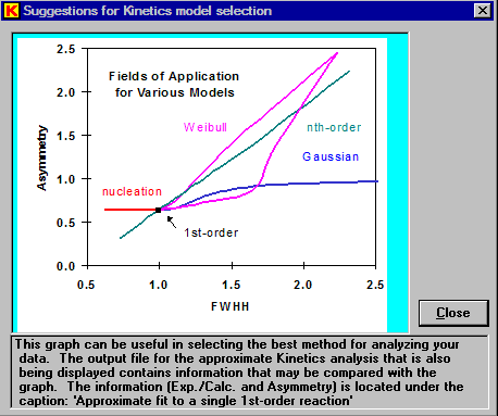
After selection of the data files, clicking the ”Next” button causes a series of approximate analyses to be done, when possible. Here is part of the results that are displayed and may be helpful in revising the initial choice of the principle analysis model that was made in the previous window, in which case the ”Back” button can be used to change that choice. The experimental and calculated FWHH (full width at half height) and the asymmetry of the reaction peak are also helpful in suggesting which model to use, by clicking the ”Suggestions” button at the bottom of the page.
For example, clicking the ”Suggestions” button gives this standard plot of reaction peak asymmetry as a function of experimental FWHH / calculated FWHH for the main domains of various models. For the current data being analyzed, a ”Gaussian” model is suggested by the average values of asymmetry ranging between 0.978 and 1.161 and the FWHH ratio ranging between 1.48 and 1.59. We chose the ”Discrete” model, which is quite similar to the ”Gaussian” model, but capable of giving a better fit, albeit with more parameters.
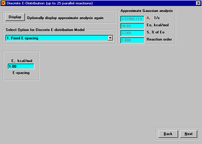
Closing the ”Suggestions” window and Clicking the ”Next” button in the previous window, permits entry of various options for doing the ”Discrete” analysis. When possible, the simplest option 1 using fixed E-spacing should be selected, because it give the greatest flexibility in determining the fit. Up to 25 parallel reactions can be used in the fitting procedure and a spacing of 1 kcal/mol will usually span most reaction peaks. If not, a larger E-spacing value can be used. Clicking the ”Next” button initiates the Kinetics calculation and displays the graph of the results.
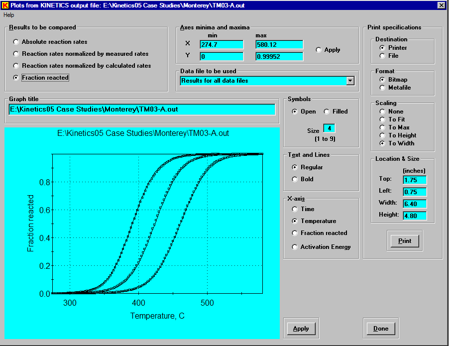
This window shows the default graph of normalized reaction rate as a function of temperature, which is the best choice for constant heating rate experiments. This default graph shows the results for all data files used in the calculation. If desired the graph for a single experiment can be selected from the drop-down list ”Data file to be used”. Various axis properties can also be set to improve the appearance of the graphs. The displayed graph(s) can be printed either directly to a printer or to a file (bitmap or metafile format) for later viewing or printing. Instead of plotting the relative reaction rate (normalized by either measured rates or calculated rates), either the fraction reacted or the absolute reaction rate (fraction reacted per unit time) can be displayed.
For example, the following is the graph of measured and calculated fraction reacted as a function of temperature.
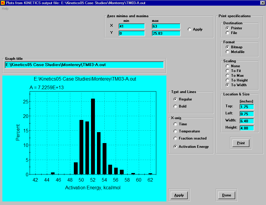
Another useful feature for the ”Discrete” kinetics model is to select ”Activation Energy” for the X axis, resulting in the following graph.
Clicking the ”Done” button in the graph window will display the main control window for the Analysis Mode. Now that the calculation has been completed, all of the control buttons have become enabled. At this point, the ”Output” button can be used to display or print the output file from the analysis that was just completed. The ”Graph” button can be used to again display the default graph or other graphs of the results. If desired, the ”Setup” button can be used to revise the nature of the calculation for the given command file. The ”Filename” button can be used to create or select a completely different command file.


