In the Data Mode, Kinetics2015 can be used to view, modify, transform, and reduce kinetic input files from pyrolysis instruments such as Wildcat Technologies HAWKⓇ, Rock-EvalⓇ, PyromatⓇ, and Thermal Analysis data (TGA, DTA, and DSC). Other data such as fraction reaction results derived from hydrous pyrolysis, MicroScale Sealed Vessel (MSSV), or other closed system pyrolysis experiments can be readily processed in the Kinetics2015 software. This module will put the data in the standard format required by Kinetics05 (see Structure of Input Data Files).
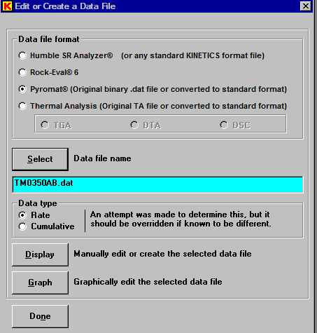
The type of data should first be selected by setting the appropriate radio button. In this example, we will use a Pyromat data file that has already been converted to standard text format [John G. Reynolds, Alan K. Burnham, and Thomas O. Mitchell, ”Kinetic analysis of California petroleum source rocks by programmed temperature pyrolysis”, Org. Geochem. Vol. 23, No. 2, pp. 109-120, 1995].
The data file name is entered by means of the Select button. An attempt is made to determine whether the data are reaction rates or cumulative reacted. It should be overridden, if the data are known to be different.
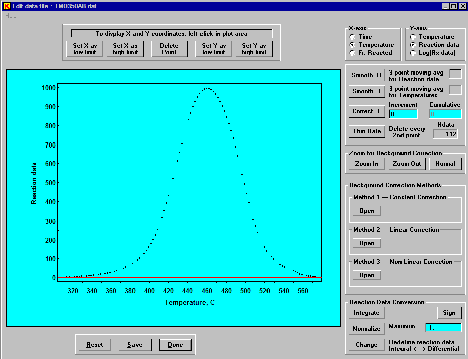
Clicking the Graph button displays the following graph of the data and the tools to maniuplate the data.
The controls at the very top of the graph permit setting lower and upper limits for the X and Y data. The controls to the upper-right of the graph permit selection of which X and Y data are displayed.
The data can be smoothed and thinned. Temperatures may be adjusted or corrected. For example, data from Rock EvalⓇ II instruments, that typically require a 35-40 oC temperature correction from nominal to true in-sample temperature, can easily be corrected using the Correct T option. If desired, the data can be integrated, differentiated, and normalized. These functions are particularly useful in processing TGA data. Any modifications can be undone using the Reset option before saving a file.
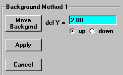
Baselines can be adjusted by first clicking the ”Open” button for one of the three methods. In the first background correction method the baseline can be moved up or down by selected increment.
In the second background correction method two points (x1, y1) and (x2,y2) can be defined by clicking on those graphical points or by manually entering the values to define a non-constant, linear baseline.
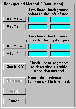
In the third background correction method, a non-linear baseline can be defined. One linear baseline is defined to left of the peak and another linear baseline is defined to the right of the peak. Then, clicking ”Check X,Y” will check the linear segments to determine a suitable transition method for connecting the two segments. A simple sigmoidal connection might be suggested. Alternatively, a spline interpolation for a convex or concave connection might be implemented. Once the ”Generate” button has become enabled, it may be clicked to generate the nonlinear background for inspection. If it is deemed suitable, the ”Apply” button can be clicked to accept it.
When editing of the data is finished, the ”Save” command will save the edited data to a user-selected file folder and file name, which may be the same name as the unedited file or a new name. At any time during the editing procedure the ”Reset” command can restore the data to the structure it had upon entering the editing window. Finally, clicking ”Done” will close the editing window.
Upon returning to the main file selection window the saved file name will appear in the ”Select” text box. It can then be displayed by clicking the ”Display” button for inspection or manual editing or it can be further graphically edited by clicking the ”Graph” button.
For example, this is the initial section of the edited file displayed in Notepad upon clicking the ”Display” button.


