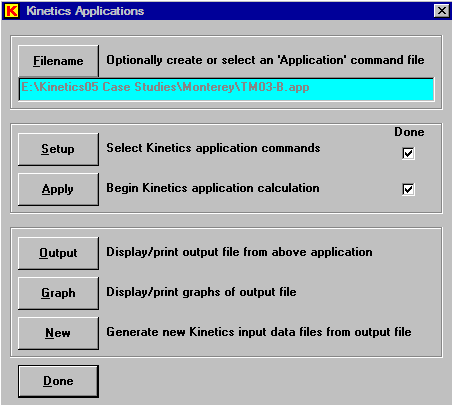
The function of the Apply Mode is to calculate reaction rates and cumulative reaction for a selected kinetics model for a user-defined thermal history.
The first step in the Apply Mode is to click ”Filename” to specify the name of the file that will contain the commands needed for the application. This file may be an existing one or it may be a new one to be created. It will be written as a text file. Conventionally, we have used ”app” or ”apl” as the file extension for this command file, but it is not required.
If the specified ”app” file is new, the ”Apply” button will not be enabled until the ”Setup” has completed. Similarly, the ”Output”, ”Graph”, and ”New” buttons will not be enabled until the application calculations are successfully completed. If the specified ”app” file already exists, the ”Apply” button will already be enabled. However, the ”Setup” function can still be used to either view or change the settings. Also, if the application calculations were previously completed for the specified ”app” file, the ”Output”, ”Graph”, and ”New” buttons buttons will already be enabled.
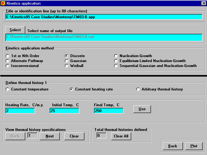
Clicking the ”Setup” button in the above window, will display the following window. The first step is to enter the Title or identification line to be used in the output files. By default this line is simply the file path and file name of the input command file, but it may be changed. The second step is to use the ”Select” button to enter the name of the output text file. Conventionally, we have used ”out” as the file extension for this file, but it is not required.
There are a nine principal kinetics application models that can be used. These are discussed in the Features window. A method should be selected for which all the kinetics parameters have already been determined. In this case we will select the ”Discrete” model, for which the kinetics parameters were just determined for Monterey Shale.
The thermal history can be constant temperature, constant heating rate, or an arbitrary thermal history. The latter is defined by time and temperature entries in a text file. One or more thermal histories can be defined for a given calculation, giving one or more curves in the resulting graph. This example will use a single thermal history for the constant heating rate conditions shown below.
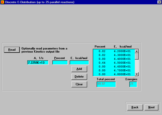
Clicking the ”Plot” button in the preceding window will then display the window for setting the kinetics parameters for the selected model, in this case the ”Discrete” model. The parameters can be manually entered. An easier method, however, is to use the ”Read” button to read the kinetics parameters from a previous output file of an Analysis Mode calculation.
Thus, reading the kinetics parameters from the output file TM03-A.out will automatically enter the needed kinetics parameters.
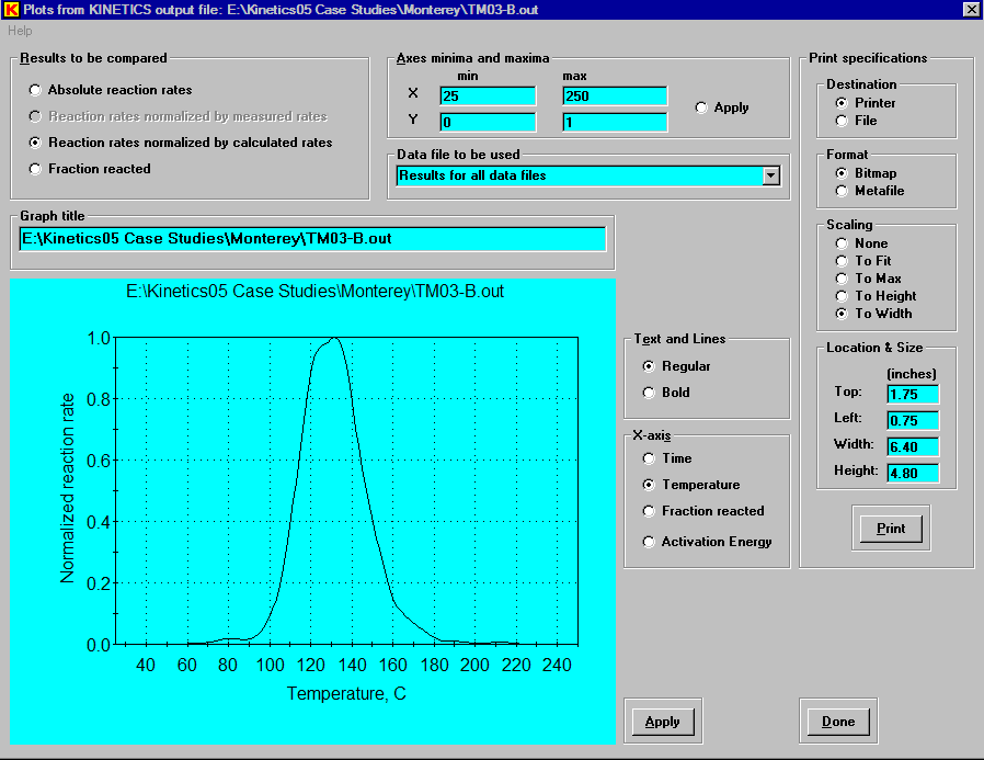
Clicking the ”Next” button in the above window then displays the default graph of the application calculation. As in the Analysis Mode, there are other selections for changing the nature of the display.
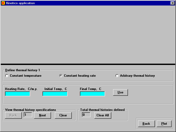
By clicking the ”Apply” button in the above window, a new thermal history can be defined and calculated for the same set of kinetics parameters in the following window.
When the graphing window is closed, the main control window for the Apply Mode is again displayed, as shown below. Now that the application calculation has been complelted, all of the control buttons have become enabled. At this point, the ”Output” button can be used to display or print the output file from the application that was just completed. The ”Graph” button can be used to again display the default graph or other graphs of the results. The ”New” button can be used to generate new Kinetics05 input data files from the output file of an application calculation. This is useful, if synthetic data are wanted for a prescribed thermal history for a selected kinetics model. Finally, if desired, the ”Setup” button can be used to revise the nature of the application calculation for the given command file or the ”Filename” button can be used to create or select a completely different command file.


